Chapter 7 A Closer Look at Assumptions

7.1 Intro

So far, bSims were used to make an idealized world. Real situations might be different from our assumed worlds. In this chapter, we will review how sensitive the various assumptions are, and how violating these assumptions might affect the estimates.

7.2 Prerequisites

library(bSims)                # simulations
library(detect)               # multinomial models
source("functions.R")         # some useful stuff

7.3 bSims runs

Work in pairs, each group can select an assumption:

• distance measurement error
• distance function misspecification
• effect of truncation distance, number of distance bins
• effect of total duration and time intervals
• movement
• heard vs. heard and seen
• 1st event vf 1st detection (duration, singing rate)
• spatial pattern random, uniform, clustered

Take a look at various assumptions by following these steps:

1. try to anticipate how a particular setting (violation of assumption) might affect estimates of \(\phi\), \(\tau\), and density,
2. run shiny::runApp("_shiny/bsims1.R") and play with that particular setting,
3. apply the setting to the code below and replicate the bSims landscapes (keep a reference, and add 2 values, one in the mid range and one extreme),
4. summarize/visualize how these changes affect estimates of availability, detectability and population density.

phi <- 0.5
tau <- 1
Den <- 2

tint <- c(3, 5, 10)
rint <- c(0.5, 1, 1.5, Inf)

B <- 100
l <- bsims_init()

sim_fun0 <- function() {
  a <- bsims_populate(l, density=Den)
  b <- bsims_animate(a, vocal_rate=phi)
  o <- bsims_detect(b, tau=tau)
  tr <- bsims_transcribe(o, tint=tint, rint=rint)
  estimate_bsims(tr$rem)
}
sim_fun1 <- function() {
  a <- bsims_populate(l, density=Den,
    xyfun=function(d) {
      (1-exp(-d^2/1^2) + dlnorm(d, 2)/dlnorm(2,2)) / 2
    },
    margin=2)
  b <- bsims_animate(a, vocal_rate=phi)
  o <- bsims_detect(b, tau=tau)
  tr <- bsims_transcribe(o, tint=tint, rint=rint)
  estimate_bsims(tr$rem)
}
sim_fun2 <- function() {
  a <- bsims_populate(l, density=Den,
    xyfun=function(d) {
      exp(-d^2/1^2) + 0.5*(1-exp(-d^2/4^2))
    },
    margin=2)
  b <- bsims_animate(a, vocal_rate=phi)
  o <- bsims_detect(b, tau=tau)
  tr <- bsims_transcribe(o, tint=tint, rint=rint)
  estimate_bsims(tr$rem)
}

set.seed(123)
res0 <- pbapply::pbreplicate(B, sim_fun0(), simplify=FALSE)
res1 <- pbapply::pbreplicate(B, sim_fun1(), simplify=FALSE)
res2 <- pbapply::pbreplicate(B, sim_fun2(), simplify=FALSE)

summary(summarize_bsims(res0))
summary(summarize_bsims(res1))
summary(summarize_bsims(res2))

Here are the Visual detections from the JOSM data all combined and by species:

load("_data/josm/josm.rda") # JOSM data

100*table(josm$counts$DetectType1)/sum(table(josm$counts$DetectType1))

## 
##      C      S      V 
## 17.528 79.829  2.643

aa <- table(josm$counts$SpeciesID, josm$counts$DetectType1)
bb <- aa[,"V"]/rowSums(aa)
hist(bb)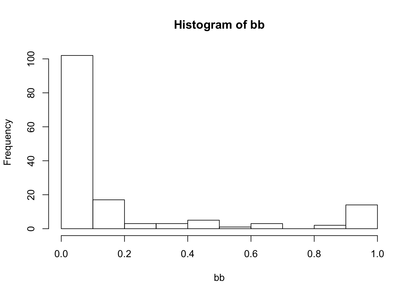

sort(bb[bb > 0.2])

##   ATTW   EAKI   TRES   BAEA   OSPR   BOGU   AMWI   MALL   MERL   RBGU 
## 0.2414 0.2500 0.2520 0.3333 0.3333 0.3663 0.4444 0.4615 0.5000 0.5000 
##   SPGR   SSHA   AMKE   BLBW   CAGU   RNDU   NOHA   BLTE   BUFF   BWTE 
## 0.5000 0.5714 0.6364 0.6452 0.6667 0.8462 0.8571 0.9310 1.0000 1.0000 
##   COGO   COHA   DCCO   GWTE   HOLA   NHOW   NSHO   RTHU   WWSC   CANV 
## 1.0000 1.0000 1.0000 1.0000 1.0000 1.0000 1.0000 1.0000 1.0000 1.0000 
##   NOPI 
## 1.0000