PVA: Publication Viability Analysis, round 3
February 06, 2018 Etc PVA publications PVAClone intrval R data cloning Hungary
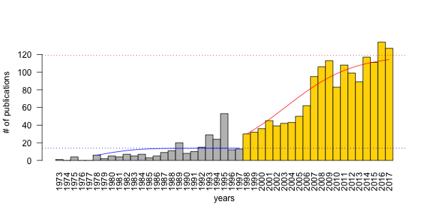
A friend and colleague of mine, Péter Batáry has circulated news from Nature magazine about the EU freezing innovation funds to Bulgaria. The article had a figure about publication trends for Bulgaria, compared with Romania and Hungary. As I have blogged about such trends in ecology before (here and here), I felt the need to update my PVA models with two years worth of data from WoS.
After downloading the yearly publications numbers
using filters ADDRESS=HUNGARY; CATEGORIES=ECOLOGY,
I started where I left off few years ago. I fit Ricker growth model
to two time intervals of the data: 1978–1997, and 1998–2017.
The R code below uses the PVAClone package that I wrote with Khurram Nadeem, and is based on fitting state-space models using MCMC and data cloning with JAGS. The other intrval package is pretty new but handy little helper (see related posts here)
library(PVAClone)
library(intrval)

## the data from WoS
x <- structure(list(years = 1973:2017, records = c(1, 0, 4, 0, 0,
    6, 2, 5, 4, 7, 5, 7, 3, 5, 9, 11, 20, 8, 10, 15, 29, 24, 53,
    12, 13, 30, 32, 36, 45, 39, 42, 43, 50, 62, 95, 106, 113, 83,
    108, 99, 89, 117, 111, 134, 127)), .Names = c("years", "records"
    ), row.names = c(NA, 45L), class = "data.frame")

## fit the 2 models
ncl <- 10 # number of clones
m1 <- pva(x$records[x$years %[]% c(1978, 1997)], ricker("none"), ncl)
m2 <- pva(x$records[x$years %[]% c(1998, 2017)], ricker("none"), ncl)

## organize estimates
cf <- data.frame(t(sapply(list(early=m1, late=m2), coef)))
cf$K <- with(cf, -a/b)

## growth curve: early period
yr1 <- 1978:1997
pr1 <- numeric(length(yr1))
pr1[1] <- log(x$records[x$years==1978])
for (i in 2:length(pr1))
    pr1[i] <- pr1[i-1] + cf["early", "a"] + cf["early", "b"]*exp(pr1[i-1])
pr1 <- exp(pr1)

## growth curve: late period
yr2 <- 1998:2017
pr2 <- numeric(length(yr2))
pr2[1] <- log(x$records[x$years==1998])
for (i in 2:length(pr2))
    pr2[i] <- pr2[i-1] + cf["late", "a"] + cf["late", "b"]*exp(pr2[i-1])
pr2 <- exp(pr2)

## and finally the figure using base graphics
op <- par(las=2)
barplot(x$records, names.arg = x$years, space=0,
    ylab="# of publications", xlab="years",
    col=ifelse(x$years < 1998, "grey", "gold"))
lines(yr1-min(x$years)+0.5, pr1, col=4)
abline(h=cf["early", "K"], col=4, lty=3)
lines(yr2-min(x$years)+0.5, pr2, col=2)
abline(h=cf["late2017", "K"], col=2, lty=3)
par(op)
Here are the model parameters for the two Ricker models:
| a | b | sigma | K | |
|---|---|---|---|---|
| 1978–1997 | 0.38 | -0.03 | 0.60 | 13.85 |
| 1998–2017 | 0.21 | 0.00 | 0.16 | 119.00 |
The K carrying capacity used to be 100 based on 1998–2012 data, but now K = 119, which is a significant improvement — heartfelt kudos to the ecologists in Hungary (more papers please)! The growth rate hasn’t changed (a = 0.21). So we can conclude that if the rate remained constant but carrying capacity increased, the change must be related to resource availability (i.e. increased funding, more jobs, improved infrastructure).
This is good news to me! Let me know what you think by leaving a comment below!
Closing the gap between data and decision making
Analyzing Ecological Data with Detection Error
This course is for researchers who analyze field observations. These data are often inconsistent because sampling protocols can change across projects, over time, or when older data are combined with new recordings.
- Analyzing Ecological Data with Detection Error
- Fitting removal models with the detect R package
- Shiny slider examples with the intrval R package
- Phylogeny and species traits predict bird detectability
- The progress bar just got a lot cheaper
ABMI (7) ARU (1) Alberta (1) BAM (1) C (1) CRAN (1) Hungary (2) JOSM (2) MCMC (2) PVA (2) PVAClone (1) QPAD (3) R (21) R packages (1) abundance (1) bioacoustics (1) biodiversity (1) birds (2) course (2) data (1) data cloning (4) datacloning (1) dclone (3) density (1) dependencies (1) detect (3) detectability (4) footprint (3) forecasting (1) functions (3) intrval (4) lhreg (1) mefa4 (1) monitoring (2) pbapply (5) phylogeny (1) plyr (1) poster (2) processing time (2) progress bar (4) publications (2) report (1) sector effects (1) shiny (1) single visit (1) site (1) slider (1) slides (2) special (3) species (1) trend (1) tutorials (2) video (4) workshop (2)