What is the cost of a progress bar in R?
September 11, 2016 Code R pbapply progress bar processing time
The pbapply R package adds progress bar to vectorized functions, like lapply. A feature request regarding progress bar for parallel functions has been sitting at the development GitHub repository for a few months. More recently, the author of the pbmcapply package dropped a note about his implementation of forking functionality with progress bar for Unix/Linux computers, which got me thinking. How should we add progress bar to snow type clusters? Which led to more important questions: what is the real cost of the progress bar and how can we reduce overhead on process times?
Parallel workflow
Fist off, let’s review how a snow type cluster works. (This is actually implemented in the parallel package, but I tend to refer to snow as that was the original package where the parallel code was taken from, see here.)
library(parallel)
parLapply
## function (cl = NULL, X, fun, ...)
## {
##     cl <- defaultCluster(cl)
##     do.call(c, clusterApply(cl, x = splitList(X, length(cl)),
##         fun = lapply, fun, ...), quote = TRUE)
## }
## <bytecode: 0x7fa43b326fc0>
## <environment: namespace:parallel>
The cl argument refers to a cluster object that can be conveniently set up via the makeCluster function. X is the ‘problem’ to be split among the workers defined by the cluster object. fun is the function that needs to be applied on elements of X. Pretty much the same as the lapply function except for the cluster argument.
Within the function, we see a nested expression that can be unpacked like this:
x <- splitList(X, length(cl))
z <- clusterApply(cl, x, fun = lapply, fun)
do.call(c, z, quote = TRUE)
The first line splits X so that it is now a list of lists. The list x is of length equal to the number of workers (i.e. length(cl)). Each element in the list x is a part of the original X vector. Let’s see how splitList works. It is an un-exported function from the parallel package that calls splitIndices. Suppose we have 10 ‘jobs’ we want to submit to 2 workers (note that these are just indices, not real values from X):
splitIndices(nx = 10, ncl = 2)
## [[1]]
## [1] 1 2 3 4 5
##
## [[2]]
## [1]  6  7  8  9 10
The first worker gets one half of the job, while the second gets the rest. In other words, the full problem is split into ncl subsets, and those are pushed to the workers in one batch. That is what the next line with clusterApply does (it uses lapply on each worker passing the function etc.). The output object z has all the results in the form of list of lists. So the final do.call expression puts together the pieces in a single list/vector that can be mapped to the input object X.
Here is example taking squares of the numbers 11:20 (note: it is good practice to stop the child processes with stopCluster when all done):
ncl <- 2
(cl <- makeCluster(ncl))
## socket cluster with 2 nodes on host 'localhost'
(X <- 11:20)
## [1] 11 12 13 14 15 16 17 18 19 20
fun <- function(x) x^2
(x <- parallel:::splitList(X, length(cl))) # these are the real values
## [[1]]
## [1] 11 12 13 14 15
##
## [[2]]
## [1] 16 17 18 19 20
str(z <- clusterApply(cl, x, fun = lapply, fun))
## List of 2
##  $ :List of 5
##   ..$ : num 121
##   ..$ : num 144
##   ..$ : num 169
##   ..$ : num 196
##   ..$ : num 225
##  $ :List of 5
##   ..$ : num 256
##   ..$ : num 289
##   ..$ : num 324
##   ..$ : num 361
##   ..$ : num 400
str(do.call(c, z, quote = TRUE))
## List of 10
##  $ : num 121
##  $ : num 144
##  $ : num 169
##  $ : num 196
##  $ : num 225
##  $ : num 256
##  $ : num 289
##  $ : num 324
##  $ : num 361
##  $ : num 400
stopCluster(cl)
Progress bar for sequential jobs
Here is a function that shows the basic principle behind the functions in the pbapply package:
library(pbapply)

pb_fun <- function(X, fun, ...) {
    X <- as.list(X) # X as list
    B <- length(X) # length of X
    fun <- match.fun(fun) # recognize the function
    out <- vector("list", B) # output list
    pb <- startpb(0, B) # set up progress bar
    for (i in seq_len(B)) { # start loop
        out[[i]] <- fun(X[[i]], ...) # apply function on X
        setpb(pb, i) # update progress bar
    } # end loop
    closepb(pb) # close progress bar on exit
    out # return output
}
The example demonstrates that the progress bar is updated at each iteration in the for loop, in this case it means 100 updates:
B <- 100
fun <- function(x) Sys.sleep(0.01)
pbo <- pboptions(type = "timer")
tmp <- pb_fun(1:B, fun)
##   |++++++++++++++++++++++++++++++++++++++++++++++++++| 100% elapsed = 01s
pboptions(pbo)
If we want to put this updating process together with the parallel evaluation, we need to split the problem in a different way. Suppose we only send one job to each worker at a time. We can do that exactly ceiling(B / ncl) times. The splitpb function takes care of the indices. Using the previous example of 10 jobs and 2 workers, we get:
splitpb(nx = 10, ncl = 2)
## [[1]]
## [1] 1 2
##
## [[2]]
## [1] 3 4
##
## [[3]]
## [1] 5 6
##
## [[4]]
## [1] 7 8
##
## [[5]]
## [1]  9 10
This gives us 10/2 = 5 occasions for updating the progress bar. And it also means that we will increase communication overhead for our parallel jobs 5-fold (from 1 to 5 batches). The overhead increases linearly with problem size B as opposed to being constant.
The cost of the progress bar
To get a sense of the overhead cost associated with the progress bar, here is a prototype function that I used for the developmental version of the pbapply package. The pbapply_test function takes some of the arguments we have covered before (X, FUN, cl). The only new argument is nout which is the maximum number of splits we allow in splitpb. nout = NULL is the default which gives exactly ceiling(nx / ncl) splits. See what happens when we cap that at 4:
splitpb(nx = 10, ncl = 2, nout = 4)
## [[1]]
## [1] 1 2 3 4
##
## [[2]]
## [1] 5 6 7 8
##
## [[3]]
## [1]  9 10
pbapply_test exposes the nout argument so that we can see what happens when we cap the number of progress bar updates (use 100 and 1) vs. we keep the updates increasing with B (NULL).
pblapply_test <-
function (X, FUN, ..., cl = NULL, nout = NULL)
{
    FUN <- match.fun(FUN)
    if (!is.vector(X) || is.object(X))
        X <- as.list(X)
    ## catch single node requests and forking on Windows
    if (!is.null(cl)) {
        if (inherits(cl, "cluster") && length(cl) < 2L)
            cl <- NULL
        if (!inherits(cl, "cluster") && cl < 2)
            cl <- NULL
        if (!inherits(cl, "cluster") && .Platform$OS.type == "windows")
            cl <- NULL
    }
    do_pb <- dopb()
    ## sequential evaluation
    if (is.null(cl)) {
        Split <- splitpb(length(X), 1L, nout = nout)
        B <- length(Split)
        if (do_pb) {
            pb <- startpb(0, B)
            on.exit(closepb(pb), add = TRUE)
        }
        rval <- vector("list", B)
        for (i in seq_len(B)) {
            rval[i] <- list(lapply(X[Split[[i]]], FUN, ...))
            if (do_pb)
                setpb(pb, i)
        }
    ## parallel evaluation
    } else {
        ## snow type cluster
        if (inherits(cl, "cluster")) {
            Split <- splitpb(length(X), length(cl), nout = nout)
            B <- length(Split)
            if (do_pb) {
                pb <- startpb(0, B)
                on.exit(closepb(pb), add = TRUE)
            }
            rval <- vector("list", B)
            for (i in seq_len(B)) {
                rval[i] <- list(parallel::parLapply(cl, X[Split[[i]]], FUN, ...))
                if (do_pb)
                    setpb(pb, i)
            }
        ## multicore type forking
        } else {
            Split <- splitpb(length(X), as.integer(cl), nout = nout)
            B <- length(Split)
            if (do_pb) {
                pb <- startpb(0, B)
                on.exit(closepb(pb), add = TRUE)
            }
            rval <- vector("list", B)
            for (i in seq_len(B)) {
                rval[i] <- list(parallel::mclapply(X[Split[[i]]], FUN, ...,
                    mc.cores = as.integer(cl)))
                if (do_pb)
                    setpb(pb, i)
            }
        }
    }
    ## assemble output list
    rval <- do.call(c, rval, quote = TRUE)
    names(rval) <- names(X)
    rval
}
The next function is test_fun which has a type argument that affects the type of progress bar. We will compare the following three types:
"none": no progress bar updates, but the function does everything else the same way including splitting;"txt": text progress bar showing percent of jobs completed;"timer": timer progress bar showing percent of jobs completed with time estimates and final elapsed time.
The no-progress bar case ("none") with nout = 1 will serve as baseline as in this case the function falls back to lapply and its parallel equivalents (parLapply and mclapply).
timer_fun <- function(X, FUN, type = "timer") {
    pbo <- pboptions(type = type)
    on.exit(pboptions(pbo))
    rbind(
        pb_NULL = system.time(pblapply_test(X, FUN, nout = NULL)),
        pb_100  = system.time(pblapply_test(X, FUN, nout = 100)),
        pb_1    = system.time(pblapply_test(X, FUN, nout = 1)),

        pb_cl_NULL = system.time(pblapply_test(X, FUN, cl = cl, nout = NULL)),
        pb_cl_100  = system.time(pblapply_test(X, FUN, cl = cl, nout = 100)),
        pb_cl_1    = system.time(pblapply_test(X, FUN, cl = cl, nout = 1)),

        pb_mc_NULL = system.time(pblapply_test(X, FUN, cl = ncl, nout = NULL)),
        pb_mc_100  = system.time(pblapply_test(X, FUN, cl = ncl, nout = 100)),
        pb_mc_1    = system.time(pblapply_test(X, FUN, cl = ncl, nout = 1))
    )
}
Here is the setup: 1000 iterations, 2 workers, and the function fun2. This function calls Sys.sleep and returns the squared value of the input. Once we open the cluster connection, run timer_fun with different settings and stop the cluster, we also call the pbmclapply function from the pbmcapply package for comparison and calculate a minimum expected time based on the fact that 0.01 * B = 10 sec.
ncl <- 2
B <- 1000
fun2 <- function(x) {
    Sys.sleep(0.01)
    x^2
}

cl <- makeCluster(ncl)
timer_out <- list(
    none  = timer_fun(1:B, fun2, type = "none"),
    txt   = timer_fun(1:B, fun2, type = "txt"),
    timer = timer_fun(1:B, fun2, type = "timer"))
stopCluster(cl)

library(pbmcapply)
tpbmc <- system.time(pbmclapply(1:B, fun, mc.cores = ncl))

tex <- 0.01 * B
tpb <- cbind(timer_out[[1]][1:3,3],
    timer_out[[2]][1:3,3],
    timer_out[[3]][1:3,3])
tcl <- cbind(timer_out[[1]][4:6,3],
    timer_out[[2]][4:6,3],
    timer_out[[3]][4:6,3])
tmc <- cbind(timer_out[[1]][7:9,3],
    timer_out[[2]][7:9,3],
    timer_out[[3]][7:9,3])
colnames(tpb) <- colnames(tcl) <- colnames(tmc) <- names(timer_out)

op <- par(mfrow = c(1, 3), las = 1, mar = c(5, 5, 2, 2))
matplot(c(B, 100, 1), tpb,
    type = "l", lty = 1, ylim = c(0, max(tpb, tcl, tmc)),
    xlab = "# pb updates", ylab = "proc time (sec)", main = "sequential")
abline(h = tex, lty = 2, col = 1)
matplot(c(B/ncl, 100, 1), tcl,
    type = "l", lty = 1, ylim = c(0, max(tpb, tcl, tmc)),
    xlab = "# pb updates", ylab = "proc time (sec)", main = "cluster")
abline(h = tex / ncl, lty = 2, col = 1)
matplot(c(B/ncl, 100, 1), tmc,
    type = "l", lty = 1, ylim = c(0, max(tpb, tcl, tmc)),
    xlab = "# pb updates", ylab = "proc time (sec)", main = "forking")
abline(h = tex / ncl, lty = 2, col = 1)
abline(h = tpbmc[3], lty = 2, col = 2)
legend("bottomleft", bty = "n", lty = c(1, 1, 1, 2, 2), col = c(1:3, 1, 2),
    legend = c(names(timer_out), "minimum", "pbmclapply"))
    par(op)
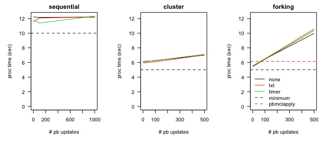
Conclusions
Here is the summary based on the plots (note: some variation exists from one run to another):
- the type of the progress bar did not affect timing results;
- the sequential runs revealed no huge effect of number of updates on processing times (a minimal effect is visible though);
- the parallel runs showed a linear relationship between number of updates and processing times;
- impact on processing times was greater when using forking mechanism.
It is clear from the results that the time required for updating/printing the progress bar is not the real bottleneck. If it was the bottleneck, we would see differences between the types. Moreover, event the "none" type led to worse performance when running in parallel. It is the increased communication overhead that is driving the timings, i.e. how many times we split-pass-collect the jobs. The situation is worst when using forking where we fork the child processes and close them multiple times. In the snow cluster case the processes are established once outside the iterative procedure therefore the smaller overhead. The pbmclapply function performs well because it uses future expectations without creating multiple forking processes (i.e. no unnecessary splits introduced).
Splitting the problem too many times severely impacts performance. It is thus a good idea to cap the number of progress bar updates when running in parallel. Another consideration in favor of this is that sometimes too many updates (i.e. tens of thousands) can clear the console output (similarly to cat("\014"), the equivalent of Ctrl+L). To prevent that, capping the number of updates could be helpful again. For example, updating 10 thousand times is pointless when results (percentage etc.) do not change much. It is like going beyond 24 frames per second for an animation: no one can recognize the difference but it makes production more expensive.
As a compromise, I came up with nout = 100 as a default value being stored as part of the progress bar options (pboptions). If one wishes to play slow-motion with the progress bar use the following line:
pboptions(nobs = NULL)
Those users who are desperate to see a progress bar while running parallel jobs, it is now available in the GitHub repository. More testing and fine tuning is required before the update finds its way to the master branch and ultimately to CRAN. In the meantime, check it out as:
devtools::install_github("psolymos/pbapply", ref = "pb-parallel")
Please provide feedback either in the comments or on GitHub.
UPDATE 2016/09/26
pbapply version 1.3-0 just made its way to CRAN.
Closing the gap between data and decision making
Analyzing Ecological Data with Detection Error
This course is for researchers who analyze field observations. These data are often inconsistent because sampling protocols can change across projects, over time, or when older data are combined with new recordings.
- Analyzing Ecological Data with Detection Error
- Fitting removal models with the detect R package
- Shiny slider examples with the intrval R package
- Phylogeny and species traits predict bird detectability
- PVA: Publication Viability Analysis, round 3
ABMI (7) ARU (1) Alberta (1) BAM (1) C (1) CRAN (1) Hungary (2) JOSM (2) MCMC (2) PVA (2) PVAClone (1) QPAD (3) R (21) R packages (1) abundance (1) bioacoustics (1) biodiversity (1) birds (2) course (2) data (1) data cloning (4) datacloning (1) dclone (3) density (1) dependencies (1) detect (3) detectability (4) footprint (3) forecasting (1) functions (3) intrval (4) lhreg (1) mefa4 (1) monitoring (2) pbapply (5) phylogeny (1) plyr (1) poster (2) processing time (2) progress bar (4) publications (2) report (1) sector effects (1) shiny (1) single visit (1) site (1) slider (1) slides (2) special (3) species (1) trend (1) tutorials (2) video (4) workshop (2)