Trends in daily R package downloads

August 23, 2016 Code R CRAN trend forecasting

This post was prompted by this blog about using the cranlogs package by Gabor Csardi. But my own interest as long time package developer dates back to this post by Ben Bolker. I like to see that my packages are being used. So I thought why stop at counting downloads and plotting the past. Why not predict into the future?

The R language has seen steady growth over the past decade in terms of its use relative to other programming languages and the number of available extension packages, both reflecting increasing community engagement. It is thus interesting to have a look at how individual packages perform over time based on CRAN download statistics.

As the R user community expands, the disparity between more and less popular packages is expected to increase. A handful of packages are on top of the CRAN download chart harvesting most of the attention of novice R users. However, popularity and trending based on downloads is not necessarily the best measure of overall impact, more like a measure that is easiest to quantify. At least I like to think that 100 downloads with 10 users is way better than 100 downloads with a single user. These two scenarios are hard to tell apart though. So for now, let’s assume that download statistics reflect real impact.

So I wanted to look at temporal patterns in the past 3 years’ download statistics from RStudio CRAN mirror for individual R packages. I quantified past trend based on fitting a log-linear glm model to counts vs. dates. Then I used the forecast package by Rob Hyndman to make short-term forecast based on an additive non-seasonal exponential smoothing model. Here is the plot_pkg_trend function:

library(cranlogs)
library(forecast)

plot_pkg_trend <-
function(pkg)
{
    op <- par(mar = c(3, 3, 1, 1) + 0.1, las = 1)
    on.exit(par(op))
    ## grab the data
    x <- cran_downloads(pkg, from = "2013-08-21", to = "2016-08-19")
    x$date <- as.Date(x$date)
    x$std_days <- 1:nrow(x) / 365
    ## past trend
    m <- glm(count ~ std_days, x, family = poisson)
    tr_past <- round(100 * (exp(coef(m)[2L]) - 1), 2)
    ## future trend
    s <- ts(x$count)
    z <- ets(s, model = "AAN")
    f <- forecast(z, h=365)
    f$date <- seq(as.Date("2016-08-20"), as.Date("2017-08-19"), 1)
    tr_future <- round(100 * (f$mean[length(f$mean)] / f$mean[1L] - 1), 2)
    ## plot
    plot(count ~ date, x, type = "l", col = "darkgrey",
        ylab = "", xlab = "",
        ylim = c(0, quantile(x$count, 0.999)),
        xlim = c(x$date[1L], as.Date("2017-08-19")))
    lines(lowess(x$date, x$count), col = 2, lwd = 2)
    polygon(c(f$date, rev(f$date)),
        c(f$upper[,2L], rev(f$lower[,2L])),
        border = NA, col = "lightblue")
    lines(f$date, f$mean, col = 4, lwd = 2)
    legend("topleft", title = paste("Package:", pkg), bty = "n",
        col = c(2, 4), lwd = 2, cex = 1,
        legend = c(paste0("past: ", tr_past, "%"),
        paste0("future: ", tr_future, "%")))
    ## return the data
    invisible(x)
}

Next, we list the top 10 R packages from the last month:

cran_top_downloads("last-month")
##    rank  package  count       from         to
## 1     1     Rcpp 221981 2016-07-23 2016-08-21
## 2     2   digest 181333 2016-07-23 2016-08-21
## 3     3  ggplot2 170577 2016-07-23 2016-08-21
## 4     4     plyr 163590 2016-07-23 2016-08-21
## 5     5  stringi 154918 2016-07-23 2016-08-21
## 6     6  stringr 153917 2016-07-23 2016-08-21
## 7     7 jsonlite 152040 2016-07-23 2016-08-21
## 8     8 magrittr 139596 2016-07-23 2016-08-21
## 9     9     curl 134026 2016-07-23 2016-08-21
## 10   10   scales 130887 2016-07-23 2016-08-21

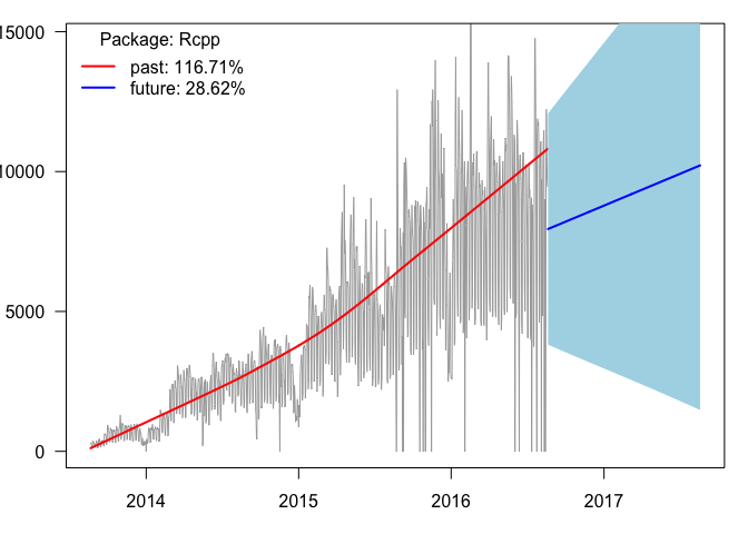
The top package was Rcpp by Dirk Eddelbuettel et al. and here is the daily trend plot with percent annual trend estimates:

plot_pkg_trend("Rcpp")

Plot 1

The increase is clear with increasing day-to-day variation suggesting that the log-linear model might be appropriate. Steady increase is predicted (the blue line starts at the last observed data point, whereas the red line is a locally weighted lowess smoothing curve on past data). The light blue 95% prediction intervals nicely follow the bulk of the zig-zagging in the observed trend.

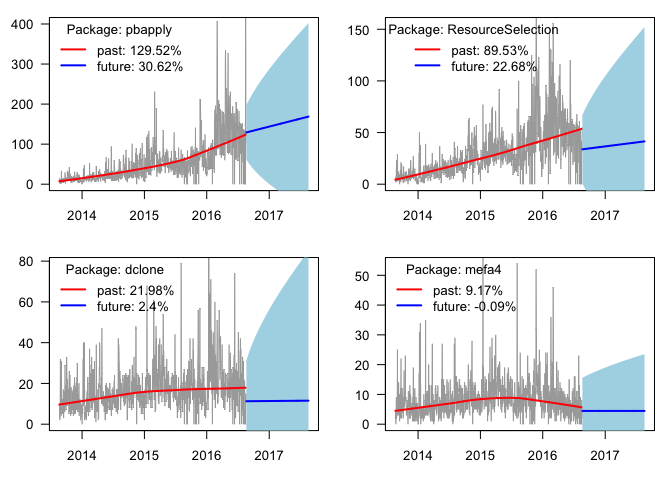
Now for my packages, here are the ones I use most often:

op <- par(mfrow = c(2, 2))
plot_pkg_trend("pbapply")
plot_pkg_trend("ResourceSelection")
plot_pkg_trend("dclone")
plot_pkg_trend("mefa4")
par(op)

Plot 2

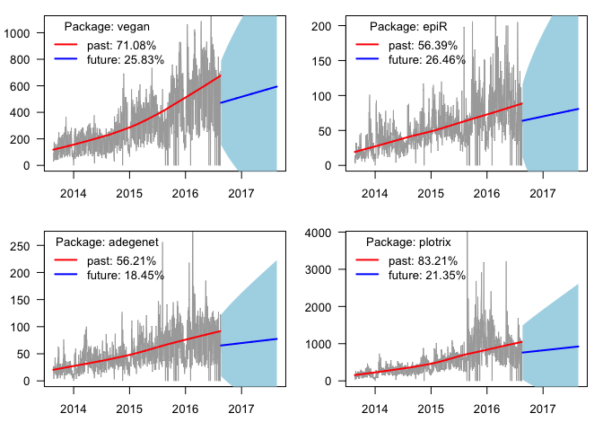
Two of them increasing nicely, the other two are showing some leveling-off. And finally, results for some packages that I am contributing to:

op <- par(mfrow = c(2, 2))
x <- plot_pkg_trend("vegan")
x <- plot_pkg_trend("epiR")
x <- plot_pkg_trend("adegenet")
x <- plot_pkg_trend("plotrix")
par(op)

Plot 3

My approach as outlined here works for packages that have been with us since 2013. However, there are packages that went extinct (orphaned, excluded from CRAN, etc.) or appeared after 2013. These need to be handled with care when comparing across many packages or changing the time horizon. If you want to take the idea presented here a step further, you can compare observed and predicted increase in downloads for many packages, or compare recent download stats and trends. Let me know what you think in the comments below!

Closing the gap between data and decision making

Follow @psolymos

CalgaryR & YEGRUG Meetup: Data Cloning - Hierarchical Models Made Easy

I moved to Canada in 2008 to start a postdoctoral fellowship with Prof. Subhash Lele at the stats department of the University of Alberta. Subhash at the time just published a paper about a statistical technique called data cloning. Data cloning is a way to use Bayesian MCMC algorithms to do frequentist inference. Yes, you read that right.

ABMI (7) ARU (1) Alberta (1) BAM (1) C (1) CRAN (1) Hungary (2) JOSM (2) MCMC (1) PVA (2) PVAClone (1) QPAD (3) R (20) R packages (1) abundance (1) bioacoustics (1) biodiversity (1) birds (2) course (2) data (1) data cloning (4) datacloning (1) dclone (3) density (1) dependencies (1) detect (3) detectability (3) footprint (3) forecasting (1) functions (3) intrval (4) lhreg (1) mefa4 (1) monitoring (2) pbapply (5) phylogeny (1) plyr (1) poster (2) processing time (2) progress bar (4) publications (2) report (1) sector effects (1) shiny (1) single visit (1) site (1) slider (1) slides (2) special (3) species (1) trend (1) tutorials (2) video (4) workshop (1)