EDMA form difference matrix

Introduction

This tutorial explains how to calculate form difference based on 2 EDMA data objects with homologous landmarks. We will use 2 data sets: one with and the other without the mutation responsible for Crouzon syndrome:

library(EDMAinR)
#> EDMAinR 0.3-0     2023-08-21

file1 <- system.file("extdata/crouzon/Crouzon_P0_Global_MUT.xyz",
    package="EDMAinR")
x1 <- read_xyz(file1)

file2 <- system.file("extdata/crouzon/Crouzon_P0_Global_NON-MUT.xyz",
    package="EDMAinR")
x2 <- read_xyz(file2)

Estimating the form matrices

We first estimate the mean forms (no bootstrap replicates are necessary).

numerator <- edma_fit(x1, B=25)
denominator <- edma_fit(x2, B=25)

Form matrices (\(FM\)) are formed as pairwise Euclidean distances between landmarks from EDMA fit objects using the estimated mean forms from objects \(A\) and \(B\).

Form difference

Form difference (\(FDM\)) is calculated as the ratio of form matrices (\(FM\)) from the numerator and denominator objects following Lele and Richtsmeier (1992, 1995): \(FDM(A,B) = FM(B)/FM(A)\).

Bootstrap distribution is based on fixing the reference \(FM\) and taking the ratio between the reference \(FM\) and the bootstrap \(FM\)s from the other object. The ref_denom argument can be used to control which object is the reference (it is the denominator by default), B is the number of replicates drawn from this distribution:

fdm <- edma_fdm(numerator, denominator, B=25)
fdm
#> EDMA form difference matrix
#> Call: edma_fdm(numerator = numerator, denominator = denominator, B = 25)
#> 25 bootstrap runs (ref: denominator)
#> Tobs = 1.5981, p < 2.22e-16

Global T-test

The global T-test is based on the pairwise distances in the \(FM\)s, taking the max/min ratio of the distances. This is then done for all the B replicates, which provides the null distribution.

Algorithm for global testing is as follows (suppose population 1 is the ‘reference’ population):

Resample \(n_1\) observations from the first sample and compute \(FM_1^*\).
Resample \(n_2\) observations from the first sample and compute \(FM_2^*\).
Compute the \(FDM^* = FM_2^* / FM_1^*\) and \(T^* = max(FDM^*) / min(FDM^*)\).
Repeat the above three steps B times to get the p-value.

global_test provides a summary of the test, plot_test helps to visualize the null distribution (histogram) and the observed T statistic (vertical line):

global_test(fdm)
#> 
#>  Bootstrap based EDMA Tobs-test
#> 
#> data:  form difference matrix
#> Tobs -value = 1.5981, B = 25, p-value < 2.2e-16
plot_test(fdm)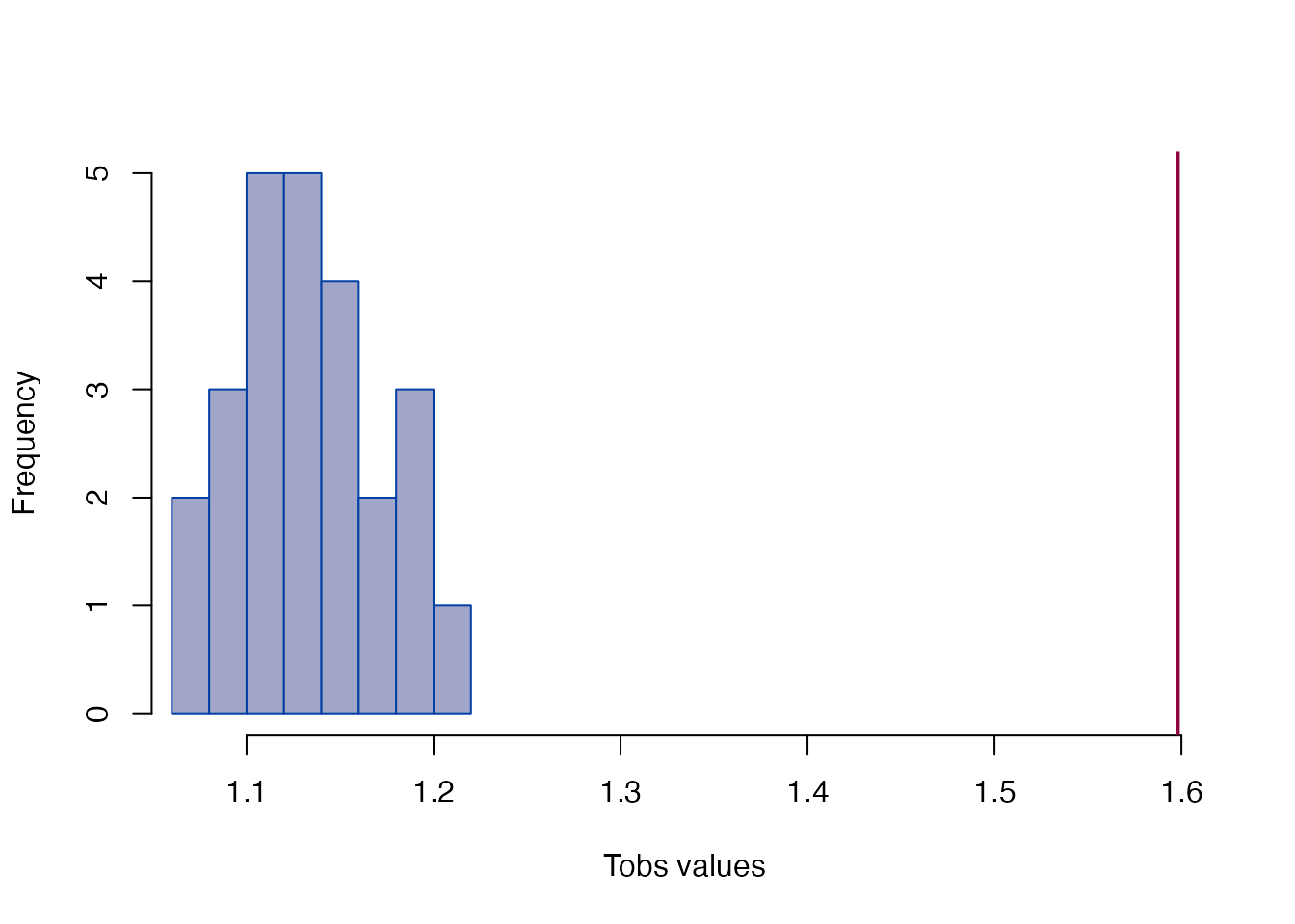

Local testing

The local testing is done based on the confidence intervals using the stacked \(FDM\)s from the bootstrap. Output structure is similar to the output of the get_fm function, but the interpretation of the confidence intervals is different due to the different nature of the bootstrap distribution. Here the distribution characterizes the \(FDM\) and not the \(FM\). The confidence level can be changed through the level argument.

The algorithm for confidence intervals for elements of the FDM is as follows:

Resample \(n_1\) observations from the first sample and compute \(FM_1^*\).
Resample \(n_2\) observations from the second sample and compute \(FM_2^*\).
Compute the \(FDM* = FM_2^* / FM_1^*\).
Repeat the above three steps B times to get the confidence intervals for the elements of the \(FDM\).

head(get_fdm(fdm))
#>     row   col      dist     lower     upper
#> 1   bas amsph 1.0425379 1.0291234 1.0572437
#> 2  cpsh amsph 0.9823765 0.9616780 0.9988809
#> 3 ethma amsph 1.0037761 0.9914403 1.0156289
#> 4 ethmp amsph 0.9401242 0.9278436 0.9510568
#> 5 laalf amsph 0.9878983 0.9788081 0.9990751
#> 6 lasph amsph 1.0161844 0.9891307 1.0317053
head(get_fdm(fdm, sort=TRUE, decreasing=TRUE))
#>       row   col     dist    lower    upper
#> 136 ethmp ethma 1.377873 1.279108 1.479039
#> 697  rpto  lpto 1.131002 1.087753 1.164933
#> 179 laalf ethmp 1.095672 1.070444 1.124045
#> 200 raalf ethmp 1.094267 1.067043 1.125650
#> 881  rpmx raalf 1.080811 1.061278 1.103610
#> 607  rpns  lpns 1.078698 1.058532 1.122745
head(get_fdm(fdm, sort=TRUE, decreasing=FALSE))
#>        row   col      dist     lower     upper
#> 527   lsqu  lpfl 0.8622059 0.8089977 0.9459507
#> 1022  rsqu  rpfl 0.8781312 0.8243285 0.9393457
#> 93   ethmp  cpsh 0.9034404 0.8810750 0.9250952
#> 212   rpsh ethmp 0.9177018 0.8965352 0.9395801
#> 190   lpsh ethmp 0.9181652 0.8947758 0.9348729
#> 4    ethmp amsph 0.9401242 0.9278436 0.9510568

Differences below or above the confidence limits indicate distances that significantly deviate from the bootstrap based null expectation, and thus are related to landmarks that drive the differences. Inspecting the highest and lowest differences (using sort) can help revealing these landmarks.

The lower and upper limits of the confidence intervals are based on confint (row names indicate the unsorted sequence of landmark pairs as in the output from get_fdm(fdm)):

head(confint(fdm))
#>                  2.5%     97.5%
#> bas-amsph   1.0291234 1.0572437
#> cpsh-amsph  0.9616780 0.9988809
#> ethma-amsph 0.9914403 1.0156289
#> ethmp-amsph 0.9278436 0.9510568
#> laalf-amsph 0.9788081 0.9990751
#> lasph-amsph 0.9891307 1.0317053

The plot_ci function shows the pairwise differences and confidence intervals. The x-axis label shows the landmark pairs, and gets really busy. Use the xshow=FALSE argument to remove labels.

plot_ci(fdm, xshow=FALSE)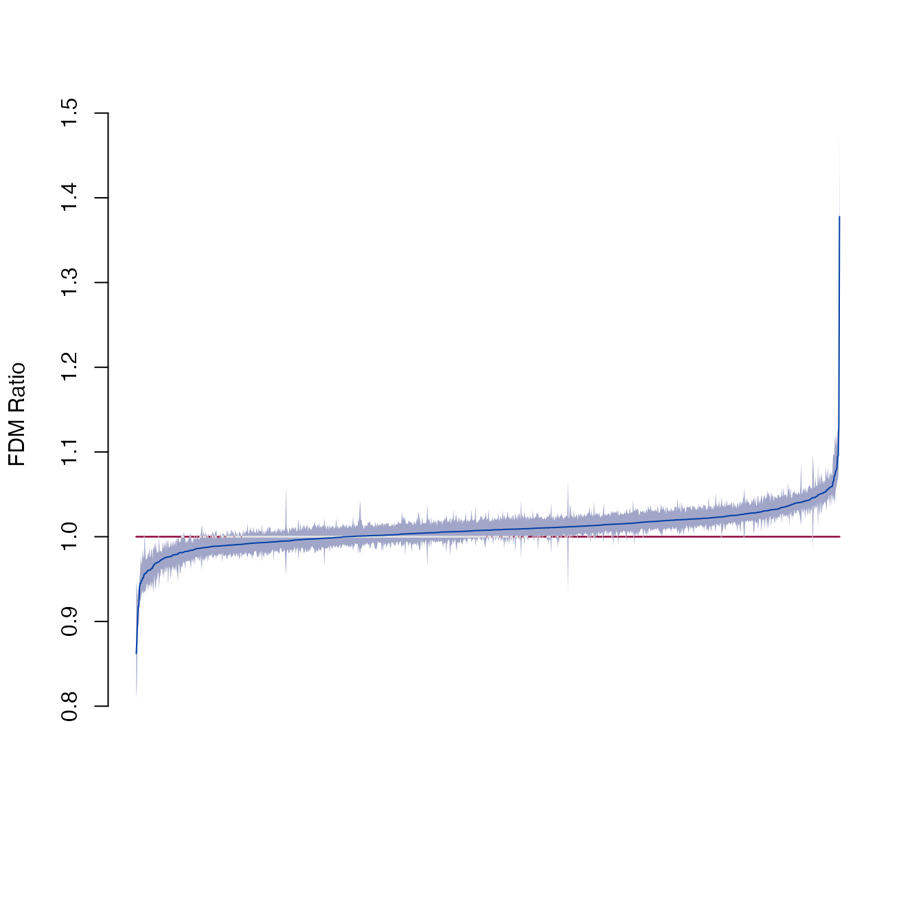

We can use the stacked \(FDM\) data frame to make a ggplot2 based plot:

library(ggplot2)
df <- get_fdm(fdm, sort=TRUE)
df$x <- 1:nrow(df) # make x-axis continuous
df$name <- paste(df$row, df$col) # add names
p <- ggplot(data=df, aes(x=x, y=dist, 
    ymin=lower, ymax=upper, label=name)) +
  geom_ribbon(col="#0000ff40", fill="#0000ff40") +
  geom_line() +
  geom_hline(yintercept=1, col=2) +
  labs(y="FDM Ratio", x="Landmark Pairs") +
  theme_linedraw() +
  theme(axis.text.x=element_blank())
p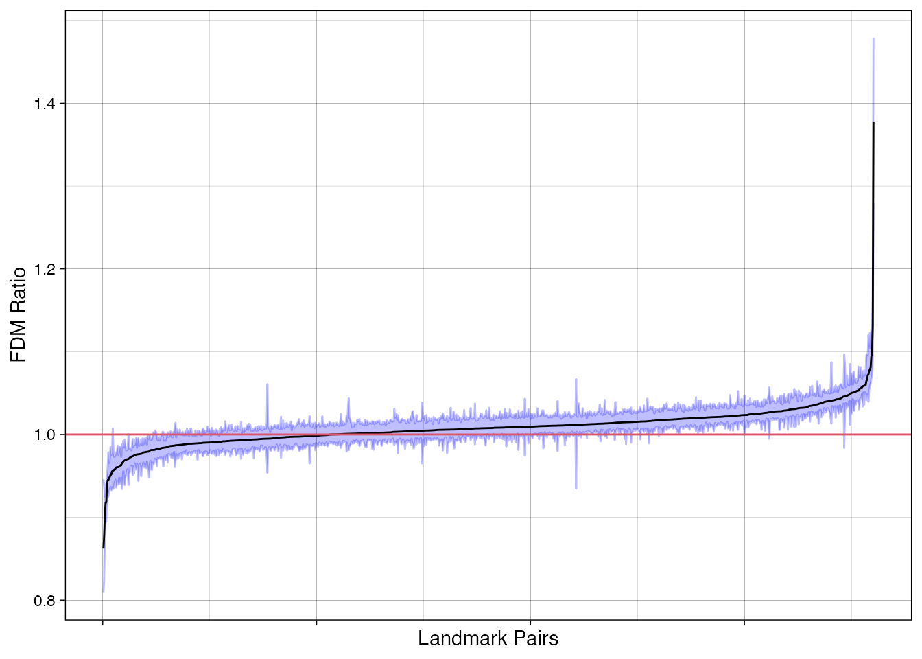

Once we have a ggplot2 version of a plot, we can load the plotly package to make the object interactive:

library(plotly)
ggplotly(p)

Influential landmarks

We can consider a landmark influential with respect to the form difference if after removing the landmark, the global T value moves close to 1. Such a case would indicate that the landmark in question is driving the form differences (i.e. pairwise distances between the landmark and other landmarks contribute to the maximum value in the T statistic). If, however, we remove a non-influential landmark, we expect the T value not to change a lot. Therefore, the ‘drop’ in the T value after removing a landmark can be used to rank landmarks based on their influence.

Influential landmarks are identified by leaving one landmark out at a time, then calculating the the T-statistic based on the remaining distances. We can use the bootstrap distribution to see of the T value ‘drop’ makes the global test non-significant. This means that after removing the landmark, the form difference cannot be distinguished from the null expectation.

The most influential landmark is the one with the largest drop in T value compared to the original T statistic. Tdrop is the newly calculated T value after leaving out the landmark in question:

infl <- get_influence(fdm)
head(infl[order(infl$Tdrop),], 10)
#>    landmark    Tdrop    lower    upper
#> 4     ethma 1.311754 1.074204 1.253519
#> 5     ethmp 1.311754 1.074204 1.253519
#> 14     lpfl 1.569097 1.074204 1.350022
#> 21     lsqu 1.569097 1.074204 1.350022
#> 1     amsph 1.598078 1.074204 1.360890
#> 2       bas 1.598078 1.074204 1.360890
#> 3      cpsh 1.598078 1.074204 1.360890
#> 6     laalf 1.598078 1.074204 1.360890
#> 7     lasph 1.598078 1.074204 1.360890
#> 8     lflac 1.598078 1.074204 1.360890

Note: we used the order function to create an index to order the rows of the infl data frame. get_influence also takes a level argument for specifying the desired confidence interval (default is 95%).

The plot function shows the landmarks ordered by Tdrop with the influential landmarks on the left-hand side of the plot. The horizontal line on the top indicates the original T value (with all the landmarks considered), the increasing line shows Tdrop, the shaded area is the null distribution for the T statistic:

plot(infl)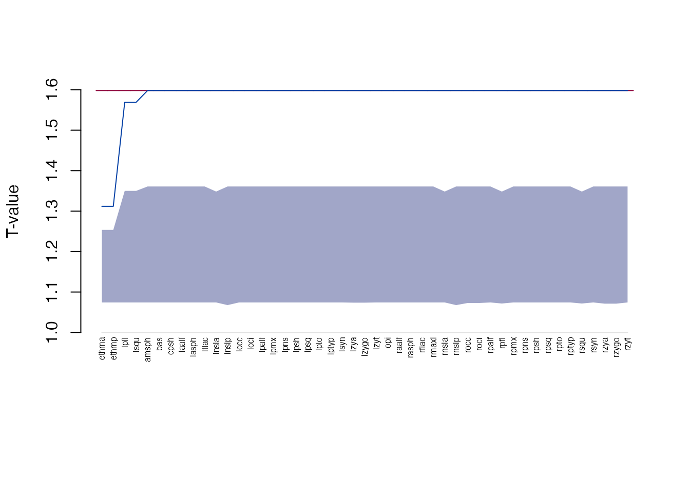

Here is the ggplot2 version:

df <- infl[order(infl$Tdrop),]
df$landmark <- factor(as.character(df$landmark), as.character(df$landmark))
p <- ggplot(data=df, aes(x=landmark, y=Tdrop, ymin=lower, ymax=upper, group=1)) +
  geom_ribbon(col="#0000ff40", fill="#0000ff40") +
  geom_hline(yintercept=global_test(fdm)$statistic, col=2) +
  geom_line() +
  labs(y="T-value", x="Landmarks") +
  theme(axis.text.x=element_text(angle = 45,
        vjust = 1, hjust=1))
p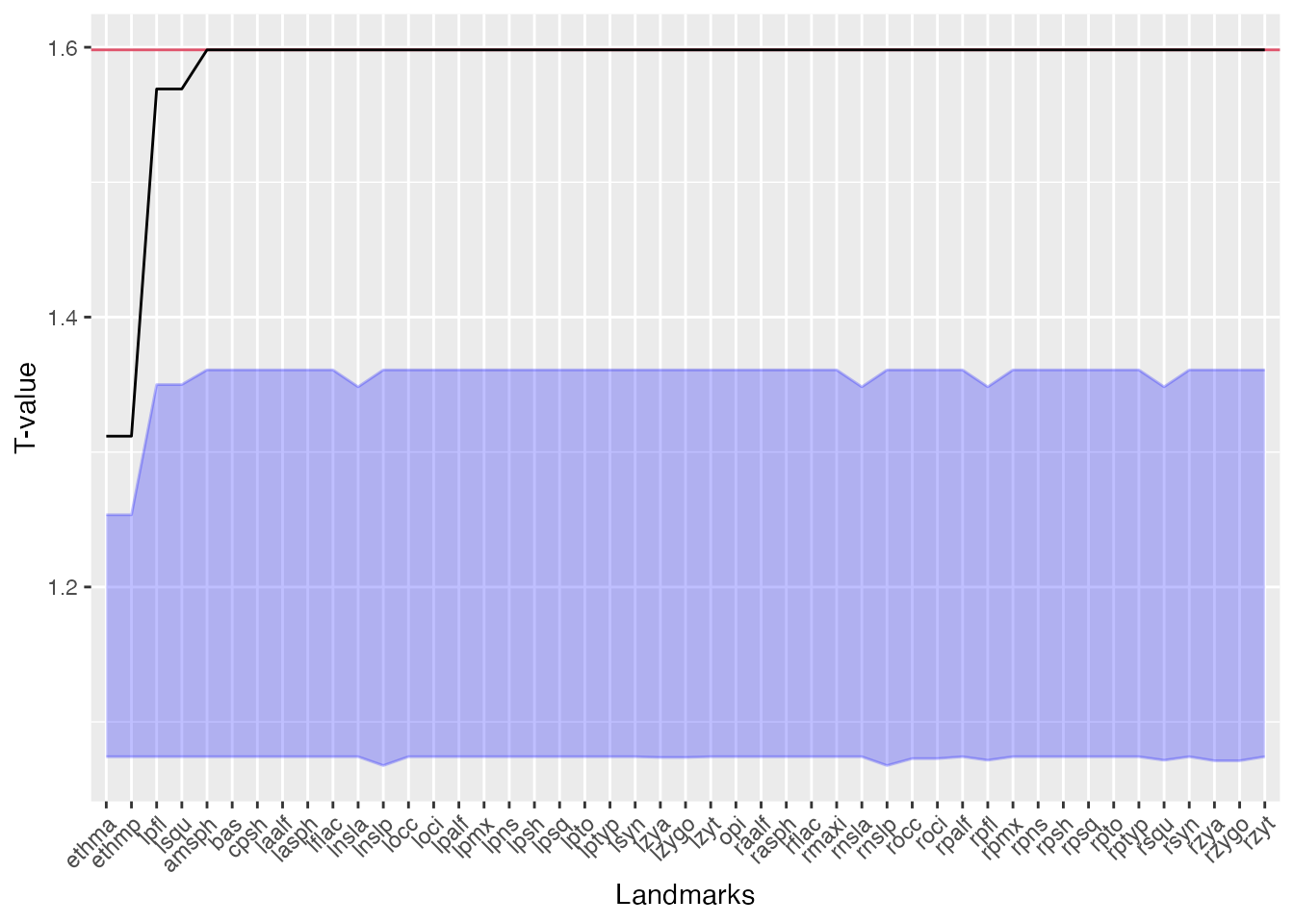

An the interactive version:

ggplotly(p)

Ordination and clustering for specimens

The ordination and cluster dendrogram shows the two sets of specimens from the 2 objects in the same diagram. The 2 sets are combined with the combine_data function:

x1
#> EDMA data: Crouzon P0 MUT
#> 47 landmarks, 3 dimensions, 28 specimens
x2
#> EDMA data: Crouzon P0 UNAFF
#> 47 landmarks, 3 dimensions, 31 specimens
(x12 <- combine_data(x1, x2))
#> EDMA data: data with 2 groups
#> 47 landmarks, 3 dimensions, 59 specimens
table(x12$groups)
#> 
#>  1  2 
#> 28 31

The visualization otherwise use the same principles as described for EDMA data objects. The difference is that the specimens and their labels are colored (using a the default qualitative palette) according to the groups (numerator vs. denominator).

If the the numerator and denominator objects are different (global T value is high, \(p\) value is low, there are influential landmarks), we expect the two groups to separate in ordination space and along the dendrogram:

plot_ord(fdm)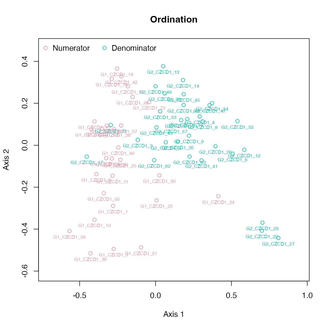

The dendrogram leaves (specimen labels) are also colored by groups:

plot_clust(fdm)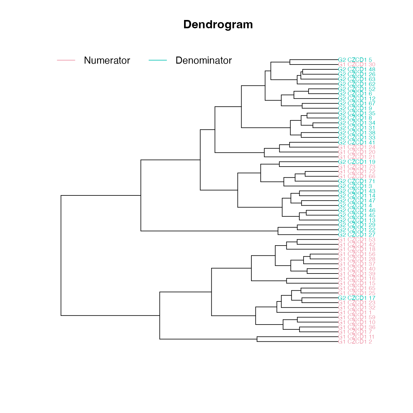

The colors can be changed via the color options:

op <- options("edma_options" = list(
    diverging = "Blue-Red",
    qualitative = "Warm"))
plot_ord(fdm)

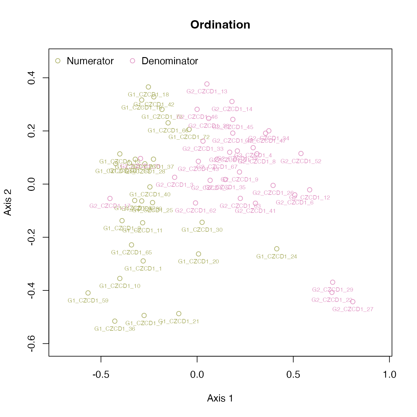
options(op)

Visualizing landmarks

The 2D and 3D plots produce a plot of the mean form from the reference object (‘prototype’). The color intensity for the landmarks (dots) is associated with the Tdrop influence value (larger the difference, the more intensive the color; red by default). Lines between the landmarks represent distances. We use the diverging palettes: <1 differences are colored blue (1st half of the palette), >1 differences are colored red (2st half of the palette).

plot_2d(fdm, cex=2)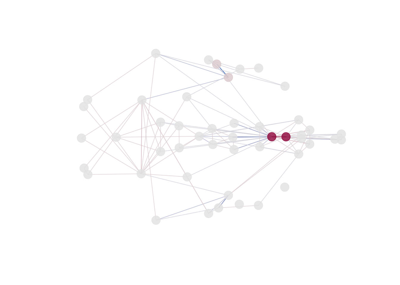

library(rgl)
xyz <- plot_3d(fdm)
text3d(xyz, texts=rownames(xyz), pos=1) # this adds names
decorate3d() # this adds the axes
rglwidget(width = 600, height = 600, reuse = FALSE)

The 2D and 3D plots do not display all the pairwise distances. If displaying all edges is desired, use the all=TRUE argument.

Peter Solymos