Progress bar overhead comparisons
October 15, 2016 Code R pbapply progress bar plyr
As a testament to my obsession with progress bars in R, here is a quick investigation about the overhead cost of drawing a progress bar during computations in R. I compared several approaches including my pbapply and Hadley Wickham’s plyr.
Let’s compare the good old lapply function from base R,
a custom-made variant called lapply_pb that was
proposed here, l_ply from the plyr package,
and finally pblapply from the pbapply package:
library(pbapply)
library(plyr)

lapply_pb <- function(X, FUN, ...) {
    env <- environment()
    pb_Total <- length(X)
    counter <- 0
    pb <- txtProgressBar(min = 0, max = pb_Total, style = 3)
    wrapper <- function(...){
        curVal <- get("counter", envir = env)
        assign("counter", curVal +1 ,envir = env)
        setTxtProgressBar(get("pb", envir = env), curVal + 1)
        FUN(...)
    }
    res <- lapply(X, wrapper, ...)
    close(pb)
    res
}

f <- function(n, type = "lapply", s = 0.1) {
    i <- seq_len(n)
    out <- switch(type,
        "lapply" = system.time(lapply(i, function(i) Sys.sleep(s))),
        "lapply_pb" = system.time(lapply_pb(i, function(i) Sys.sleep(s))),
        "l_ply" = system.time(l_ply(i, function(i)
            Sys.sleep(s), .progress="text")),
        "pblapply" = system.time(pblapply(i, function(i) Sys.sleep(s))))
    unname(out["elapsed"] - (n * s))
}
Use the function f to run all four variants. The expected run time
is n * s (number of iterations x sleep duration),
therefore we can calculate the overhead from the
return objects as elapsed minus expected. Let’s get some numbers
for a variety of n values and replicated B times
to smooth out the variation:
n <- c(10, 100, 1000)
s <- 0.01
B <- 10

x1 <- replicate(B, sapply(n, f, type = "lapply", s = s))
x2 <- replicate(B, sapply(n, f, type = "lapply_pb", s = s))
x3 <- replicate(B, sapply(n, f, type = "l_ply", s = s))
x4 <- replicate(B, sapply(n, f, type = "pblapply", s = s))

m <- cbind(
    lapply = rowMeans(x1),
    lapply_pb = rowMeans(x2),
    l_ply = rowMeans(x3),
    pblapply = rowMeans(x4))

op <- par(mfrow=c(1, 2))
matplot(n, m, type = "l", lty = 1, lwd = 3,
    ylab = "Overhead (sec)", xlab = "# iterations")
legend("topleft", bty = "n", col = 1:4, lwd = 3, text.col = 1:4,
    legend = colnames(m))
matplot(n, m / n, type = "l", lty = 1, lwd = 3,
    ylab = "Overhead / # iterations (sec)", xlab = "# iterations")
par(op)
dev.off()
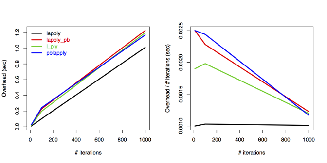
The plot tells us that the overhead increases linearly
with the number of iterations when using lapply
without progress bar.
All other three approaches show similar patterns to each other
and the overhead is constant: lines are
parallel above 100 iterations after an initial increase.
The per iteration overhead is decreasing, approaching
the lapply line. Note that all the differences are tiny
and there is no practical consequence
for choosing one approach over the other in terms of processing times.
This is good news and another argument for using progress bar
because its usefulness far outweighs the minimal
(<2 seconds here for 1000 iterations)
overhead cost.
As always, suggestions and feature requests are welcome. Leave a comment or visit the GitHub repo.
Closing the gap between data and decision making
Analyzing Ecological Data with Detection Error
This course is for researchers who analyze field observations. These data are often inconsistent because sampling protocols can change across projects, over time, or when older data are combined with new recordings.
- Analyzing Ecological Data with Detection Error
- Fitting removal models with the detect R package
- Shiny slider examples with the intrval R package
- Phylogeny and species traits predict bird detectability
- PVA: Publication Viability Analysis, round 3
ABMI (7) ARU (1) Alberta (1) BAM (1) C (1) CRAN (1) Hungary (2) JOSM (2) MCMC (2) PVA (2) PVAClone (1) QPAD (3) R (21) R packages (1) abundance (1) bioacoustics (1) biodiversity (1) birds (2) course (2) data (1) data cloning (4) datacloning (1) dclone (3) density (1) dependencies (1) detect (3) detectability (4) footprint (3) forecasting (1) functions (3) intrval (4) lhreg (1) mefa4 (1) monitoring (2) pbapply (5) phylogeny (1) plyr (1) poster (2) processing time (2) progress bar (4) publications (2) report (1) sector effects (1) shiny (1) single visit (1) site (1) slider (1) slides (2) special (3) species (1) trend (1) tutorials (2) video (4) workshop (2)