Plot or Extract Results of Constrained Correspondence Analysis or Redundancy Analysis

Functions to plot or extract results of constrained correspondence analysis (cca), redundancy analysis (rda) or constrained analysis of principal coordinates (capscale).

# S3 method for cca
plot(x, choices = c(1, 2), display = c("sp", "wa", "cn"),
     scaling = "species", type, xlim, ylim, const,
     correlation = FALSE, hill = FALSE, ...)
# S3 method for cca
text(x, display = "sites", labels, choices = c(1, 2),
     scaling = "species", arrow.mul, head.arrow = 0.05, select, const,
     axis.bp = FALSE, correlation = FALSE, hill = FALSE, ...)
# S3 method for cca
points(x, display = "sites", choices = c(1, 2),
       scaling = "species", arrow.mul, head.arrow = 0.05, select, const,
       axis.bp = FALSE, correlation = FALSE, hill = FALSE, ...)
# S3 method for cca
scores(x, choices = c(1,2), display = c("sp","wa","cn"),
       scaling = "species", hill = FALSE, ...)
# S3 method for rda
scores(x, choices = c(1,2), display = c("sp","wa","cn"),
       scaling = "species", const, correlation = FALSE, ...)
# S3 method for cca
summary(object, scaling = "species", axes = 6,
        display = c("sp", "wa", "lc", "bp", "cn"),
        digits = max(3, getOption("digits") - 3),
        correlation = FALSE, hill = FALSE, ...)
# S3 method for summary.cca
print(x, digits = x$digits, head = NA, tail = head, ...)
# S3 method for summary.cca
head(x, n = 6, tail = 0, ...)
# S3 method for summary.cca
tail(x, n = 6, head = 0, ...)

Arguments

x, object	A cca result object.
choices	Axes shown.
display	Scores shown. These must include some of the alternatives species or sp for species scores, sites or wa for site scores, lc for linear constraints or LC scores, or bp for biplot arrows or cn for centroids of factor constraints instead of an arrow, and reg for regression coefficients (a.k.a. canonical coefficients).
scaling	Scaling for species and site scores. Either species (2) or site (1) scores are scaled by eigenvalues, and the other set of scores is left unscaled, or with 3 both are scaled symmetrically by square root of eigenvalues. Corresponding negative values can be used in cca to additionally multiply results with \(\sqrt(1/(1-\lambda))\). This scaling is know as Hill scaling (although it has nothing to do with Hill's rescaling of decorana). With corresponding negative values in rda, species scores are divided by standard deviation of each species and multiplied with an equalizing constant. Unscaled raw scores stored in the result can be accessed with scaling = 0. The type of scores can also be specified as one of "none", "sites", "species", or "symmetric", which correspond to the values 0, 1, 2, and 3 respectively. Arguments correlation and hill in scores.rda and scores.cca respectively can be used in combination with these character descriptions to get the corresponding negative value.
correlation, hill	logical; if scaling is a character description of the scaling type, correlation or hill are used to select the corresponding negative scaling type; either correlation-like scores or Hill's scaling for PCA/RDA and CA/CCA respectively. See argument scaling for details.
type	Type of plot: partial match to text for text labels, points for points, and none for setting frames only. If omitted, text is selected for smaller data sets, and points for larger.
xlim, ylim	the x and y limits (min,max) of the plot.
labels	Optional text to be used instead of row names.
arrow.mul	Factor to expand arrows in the graph. Arrows will be scaled automatically to fit the graph if this is missing.
head.arrow	Default length of arrow heads.
select	Items to be displayed. This can either be a logical vector which is TRUE for displayed items or a vector of indices of displayed items.
const	General scaling constant to rda scores. The default is to use a constant that gives biplot scores, that is, scores that approximate original data (see vignette on ‘Design Decisions’ with browseVignettes("vegan") for details and discussion). If const is a vector of two items, the first is used for species, and the second item for site scores.
axis.bp	Draw axis for biplot arrows.
axes	Number of axes in summaries.
digits	Number of digits in output.
n, head, tail	Number of rows printed from the head and tail of species and site scores. Default NA prints all.
...	Parameters passed to other functions.

Details

Same plot function will be used for cca and rda. This produces a quick, standard plot with current scaling.

The plot function sets colours (col), plotting characters (pch) and character sizes (cex) to certain standard values. For a fuller control of produced plot, it is best to call plot with type="none" first, and then add each plotting item separately using text.cca or points.cca functions. These use the default settings of standard text and points functions and accept all their parameters, allowing a full user control of produced plots.

Environmental variables receive a special treatment. With display="bp", arrows will be drawn. These are labelled with text and unlabelled with points. The arrows have basically unit scaling, but if sites were scaled (scaling "sites" or "symmetric"), the scores of requested axes are adjusted relative to the axis with highest eigenvalue. With scaling = "species" or scaling = "none", the arrows will be consistent with vectors fitted to linear combination scores (display = "lc" in function envfit), but with other scaling alternatives they will differ. The basic plot function uses a simple heuristics for adjusting the unit-length arrows to the current plot area, but the user can give the expansion factor in mul.arrow. With display="cn" the centroids of levels of factor variables are displayed (these are available only if there were factors and a formula interface was used in cca or rda). With this option continuous variables still are presented as arrows and ordered factors as arrows and centroids. With display = "reg" arrows will be drawn for regression coefficients (a.k.a. canonical coefficients) of constraints and conditions. Biplot arrows can be interpreted individually, but regression coefficients must be interpreted all together: the LC score for each site is the sum of regressions displayed by arrows. The partialled out conditions are zero and not shown in biplot arrows, but they are shown for regressions, and show the effect that must be partialled out to get the LC scores. The biplot arrows are more standard and more easily interpreted, and regression arrows should be used only if you know that you need them.

If you want to have a better control of plots, it is best to construct the plot text and points commands which accept graphical parameters. It is important to remember to use the same scaling, correlation and hill arguments in all calls. The plot.cca command returns invisibly an ordiplot result object, and this will have consistent scaling for all its elements. The easiest way for full control of graphics is to first set up the plot frame using plot with type = "n" and all needed scores in display and save this result. The points and text commands for ordiplot will allow full graphical control (see section Examples).

Function summary lists all scores and the output can be very long. You can suppress scores by setting axes = 0 or display = NA or display = NULL. You can display some first or last (or both) rows of scores by using head or tail or explicit print command for the summary.

Palmer (1993) suggested using linear constraints (“LC scores”) in ordination diagrams, because these gave better results in simulations and site scores (“WA scores”) are a step from constrained to unconstrained analysis. However, McCune (1997) showed that noisy environmental variables (and all environmental measurements are noisy) destroy “LC scores” whereas “WA scores” were little affected. Therefore the plot function uses site scores (“WA scores”) as the default. This is consistent with the usage in statistics and other functions in R (lda, cancor).

Value

The plot function returns invisibly a plotting structure which can be used by function identify.ordiplot to identify the points or other functions in the ordiplot family.

See also

cca, rda and capscale for getting something to plot, ordiplot for an alternative plotting routine and more support functions, and text, points and arrows for the basic routines.

Examples

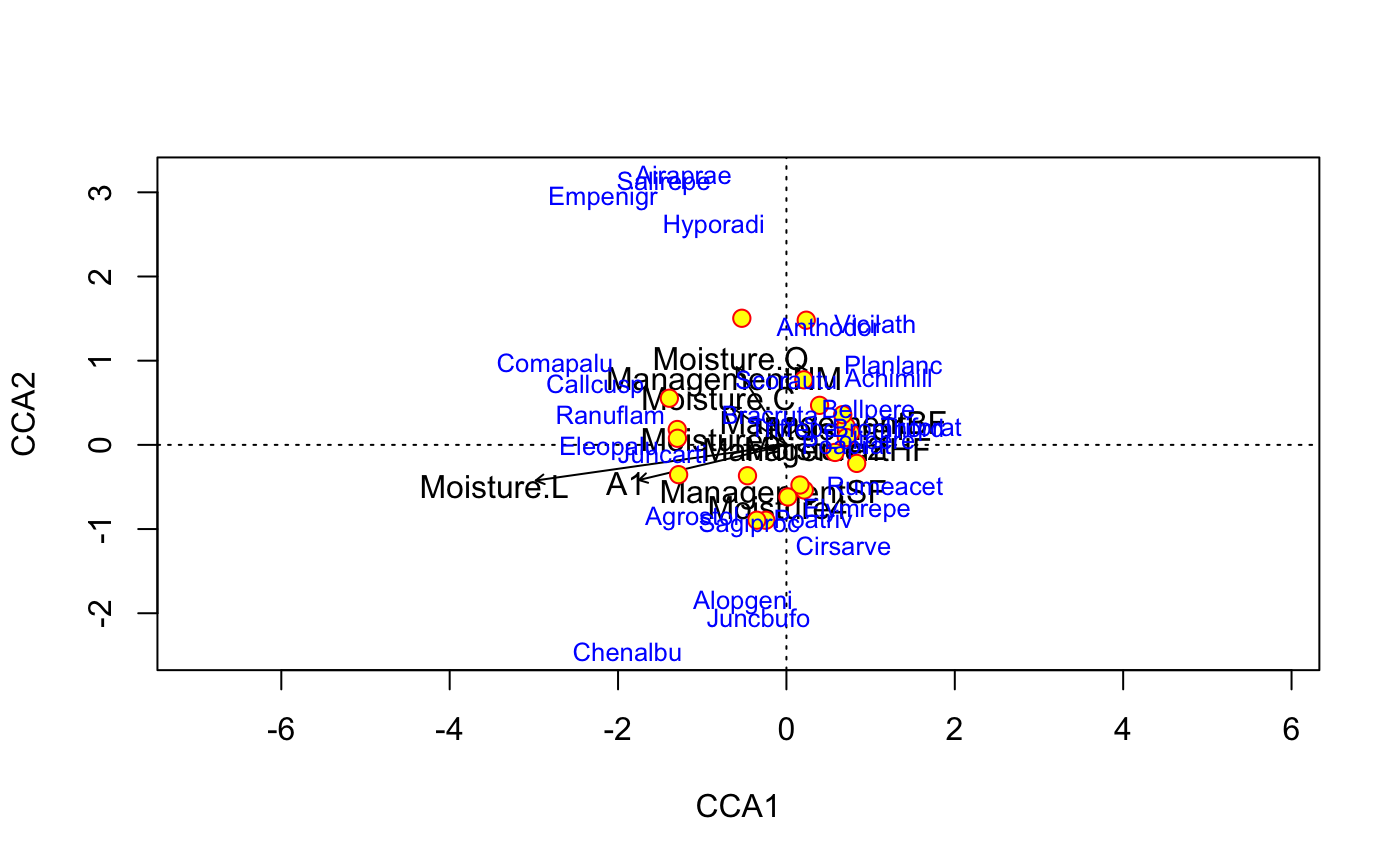
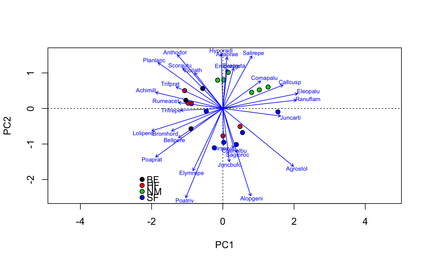
data(dune)
data(dune.env)
mod <- cca(dune ~ A1 + Moisture + Management, dune.env)
## better control -- remember to set scaling etc identically
plot(mod, type="n", scaling="sites")
text(mod, dis="cn", scaling="sites")
points(mod, pch=21, col="red", bg="yellow", cex=1.2, scaling="sites")
text(mod, "species", col="blue", cex=0.8, scaling="sites")
## catch the invisible result and use ordiplot support - the example
## will make a biplot with arrows for species and correlation scaling
pca <- rda(dune)
pl <- plot(pca, type="n", scaling="sites", correlation=TRUE)
with(dune.env, points(pl, "site", pch=21, col=1, bg=Management))
text(pl, "sp", arrow=TRUE, length=0.05, col=4, cex=0.6, xpd=TRUE)
#> Warning: "length" is not a graphical parameter
with(dune.env, legend("bottomleft", levels(Management), pch=21, pt.bg=1:4, bty="n"))
## Limited output of 'summary'
head(summary(mod), tail=2)
#> 
#> Call:
#> cca(formula = dune ~ A1 + Moisture + Management, data = dune.env) 
#> 
#> Partitioning of scaled Chi-square:
#>               Inertia Proportion
#> Total          2.1153     1.0000
#> Constrained    1.1392     0.5385
#> Unconstrained  0.9761     0.4615
#> 
#> Eigenvalues, and their contribution to the scaled Chi-square 
#> 
#> Importance of components:
#>                         CCA1   CCA2    CCA3    CCA4    CCA5    CCA6    CCA7
#> Eigenvalue            0.4483 0.3001 0.14995 0.10733 0.05668 0.04335 0.03345
#> Proportion Explained  0.2119 0.1419 0.07089 0.05074 0.02680 0.02050 0.01581
#> Cumulative Proportion 0.2119 0.3538 0.42470 0.47544 0.50223 0.52273 0.53855
#>                          CA1     CA2     CA3     CA4     CA5     CA6     CA7
#> Eigenvalue            0.3064 0.13191 0.11516 0.10947 0.07724 0.07575 0.04871
#> Proportion Explained  0.1448 0.06236 0.05444 0.05175 0.03652 0.03581 0.02303
#> Cumulative Proportion 0.6834 0.74574 0.80018 0.85194 0.88845 0.92427 0.94730
#>                           CA8     CA9     CA10     CA11     CA12
#> Eigenvalue            0.03758 0.03106 0.021024 0.012542 0.009277
#> Proportion Explained  0.01777 0.01468 0.009939 0.005929 0.004386
#> Cumulative Proportion 0.96506 0.97975 0.989685 0.995614 1.000000
#> 
#> Accumulated constrained eigenvalues
#> Importance of components:
#>                         CCA1   CCA2   CCA3    CCA4    CCA5    CCA6    CCA7
#> Eigenvalue            0.4483 0.3001 0.1499 0.10733 0.05668 0.04335 0.03345
#> Proportion Explained  0.3935 0.2635 0.1316 0.09422 0.04976 0.03806 0.02937
#> Cumulative Proportion 0.3935 0.6570 0.7886 0.88282 0.93258 0.97063 1.00000
#> 
#> Scaling 2 for species and site scores
#> * Species are scaled proportional to eigenvalues
#> * Sites are unscaled: weighted dispersion equal on all dimensions
#> 
#> 
#> Species scores
#> 
#>             CCA1    CCA2     CCA3     CCA4      CCA5     CCA6
#> Achimill  0.8150  0.4375 -0.11236  0.35595 -0.114763 -0.01972
#> Agrostol -0.7488 -0.4783  0.03561  0.17039  0.187389  0.23471
#> Airaprae -0.8186  1.7469  1.04506 -0.28593  0.191836  0.73077
#> Alopgeni -0.3442 -1.0216  0.37620  0.02296 -0.004041  0.04789
#> Anthodor  0.3367  0.7694 -0.07602 -0.05421  0.136354  0.42463
#> Bellpere  0.6535  0.2200  0.03438  0.60436 -0.090469  0.28138
#> ....                                                         
#> Bracruta -0.1309  0.2009 -0.03708 -0.17421 -0.109657  0.04381
#> Callcusp -1.5181  0.3834 -0.23255  0.15246  0.104239 -0.11424
#> 
#> 
#> Site scores (weighted averages of species scores)
#> 
#>         CCA1    CCA2     CCA3    CCA4    CCA5    CCA6
#> 1     1.2468 -0.4017  0.91955  0.7292  1.5785 -1.0196
#> 2     0.8622 -0.1641  0.25789  1.7240 -0.7592 -0.6479
#> 3     0.3165 -0.9785  0.82952  0.7451  0.6556  0.3256
#> 4     0.2405 -0.8699  1.07861  1.4103  1.1164  2.4714
#> 5     1.1362  0.2621 -1.10847 -0.9417  0.5630  1.1495
#> 6     1.0575  0.4041 -1.65035 -1.8483  1.0287 -0.1690
#> ....                                                 
#> 19   -0.7913  2.7451  2.93017 -1.3851 -0.3932  1.7277
#> 20   -2.0770  1.0113 -0.02581 -0.8949  1.6406 -1.7917
#> 
#> 
#> Site constraints (linear combinations of constraining variables)
#> 
#>         CCA1    CCA2     CCA3    CCA4    CCA5     CCA6
#> 1     0.7245 -0.3695  1.25652 -0.3678  0.9827 -0.60590
#> 2     0.9033  0.4250  0.03901  1.0557 -1.0860 -1.61234
#> 3     0.4493 -0.6694  0.67765  0.8695  0.9609  1.52307
#> 4     0.4550 -0.6532  0.72768  0.8529  0.9795  1.50218
#> 5     0.9671 -0.2010 -1.93972 -0.5807  0.2582  0.31905
#> 6     1.0805  0.1235 -0.93911 -0.9126  0.6307 -0.09863
#> ....                                                  
#> 19   -1.4581  1.6074  1.16812 -0.5305  0.3178 -0.40336
#> 20   -1.4468  1.6399  1.26818 -0.5637  0.3551 -0.44513
#> 
#> 
#> Biplot scores for constraining variables
#> 
#>                 CCA1    CCA2     CCA3     CCA4     CCA5     CCA6
#> A1           -0.5554 -0.1617 -0.67982  0.10708 -0.17998  0.30507
#> Moisture.L   -0.9437 -0.1638  0.07974 -0.02238  0.03067 -0.02368
#> Moisture.Q   -0.1876  0.3571 -0.45352 -0.17237  0.28350 -0.63025
#> Moisture.C   -0.2069  0.1732  0.10635  0.68203  0.50123  0.35887
#> ManagementHF  0.3645 -0.1171 -0.42202 -0.67746  0.17212 -0.12317
#> ManagementNM -0.5855  0.7267 -0.01115 -0.09642 -0.11445  0.27037
#> ManagementSF -0.1511 -0.6957  0.38543  0.24770  0.29469  0.23829
#> 
#> 
#> Centroids for factor constraints
#> 
#>                 CCA1     CCA2     CCA3     CCA4     CCA5    CCA6
#> Moisture1     0.9119  0.35388 -0.40013 -0.26218  0.02084 -0.4708
#> Moisture2     0.5015 -0.06706  0.60222  1.12478  0.33942  1.2024
#> Moisture4    -0.1522 -1.35873  0.76544 -1.37289 -1.80794  0.3849
#> Moisture5    -1.3394  0.11972 -0.20942  0.04843  0.39751 -0.3902
#> ManagementBF  0.8376  0.41614  0.13885  1.40679 -0.97766 -0.9604
#> ManagementHF  0.5426 -0.17426 -0.62822 -1.00848  0.25622 -0.1834
#> ManagementNM -1.1010  1.36665 -0.02097 -0.18131 -0.21523  0.5084
#> ManagementSF -0.2320 -1.06831  0.59183  0.38035  0.45250  0.3659
#> 
## Scaling can be numeric or more user-friendly names
## e.g. Hill's scaling for (C)CA
scrs <- scores(mod, scaling = "sites", hill = TRUE)
## or correlation-based scores in PCA/RDA
scrs <- scores(rda(dune ~ A1 + Moisture + Management, dune.env),
               scaling = "sites", correlation = TRUE)