Marginal Effect Plots

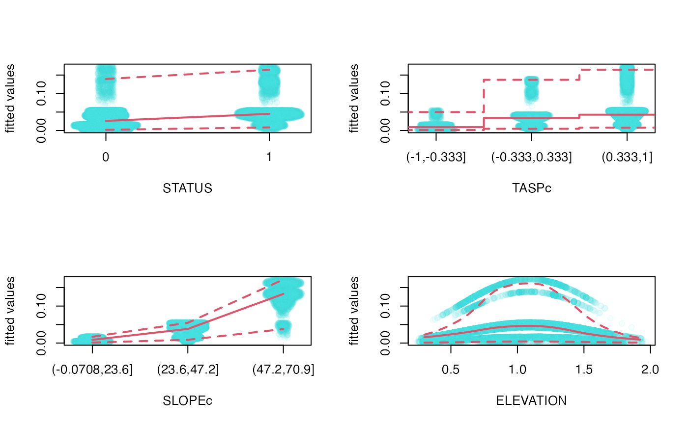
Scatterplot of marginal effects based on fitted model objects.

Usage

mep(object, ...)

# S3 method for default
mep(object, which=NULL, link=NULL,
    level=0.95, unique=10, n=25, minbucket=5, digits=4,
    col.points, col.lines=c(2, 2), pch=19, lty=c(1, 2), lwd=c(2,2),
    ask, subset=NULL, ylab, ...)

Arguments

object: a fitted model object.
which: numeric, logical, or character. Indices for the variables in the model frame if only one or a subset is desired.
link: character accepted by make.link, optional argument to determine scaling. It is guessed when value cannot be determined based on family(object)$link (see Details).
level: numeric [0, 1], the confidence level required.
unique, digits: numeric, the number of unique points above which bins are used. If the number of unique values is less than or equal to this number, unique values are used without binning. Unique values are subject to rounding to digits.
n, minbucket: number of bins (n) to be used in quantile estimation when variable is not treated as unique points. minbucket is the minimum number of points within each bin. n is decreased until minbucket condition is satisfied.
col.points, pch: color and type of points to be plotted.
col.lines, lty, lwd: color, type, and width of quantile lines to be plotted. The 1st value correspond to the median, the 2nd value to the upper and lower quantiles, respectively.
ask: logical. If TRUE, the user is asked before each plot, see par(ask=.).
subset: an optional vector specifying a subset of the data to be used for plotting.
ylab: character or expression, optional y axis label.
...: other possible arguments passed to graphical functions.

Details

The input object must have a fitted and model.frame method, and possibly a well identifiable family/link component (family(object)$link). In the absence of family/link information, the range of the fitted value will be used to guess the scaling (identity, log, or logit) unless directly supplied via the link argument.

Fitted values (f(x) = f(x_1,...,x_i,...,x_p); i = 1,...,p) are plotted against x_i. The visual display is determined by the type of x_i (un-ordered factor, ordered factor, unique numeric values, binned numeric values). For each unique vale or bin, the median and confidence intervals (quantiles corresponding to level) of f(x) are calculated. Binned values are smoothed by lowess unless n < 3.

Jitter is added to factor and unique value types. Jitter is calculated based on kernel density.

The model frame includes the response variable as well. Plotting f(x) as a function of the observations might be a useful visualization too to indicate goodness of fit or the lack of it.

Value

The produces one or several marginal plots as a side effect. Returns a list of quantiles of fitted values corresponding to binned/unique values of variables in the input object.

References

Avgar, T., Lele, S. R., Keim, J. L. & Boyce, M. S. (2017) Relative Selection Strength: Quantifying effect size in habitat- and step-selection inference. Ecology and Evolution 7, 5322--5330.

Author

Peter Solymos and Subhash Lele

Examples

data(goats)
goats$ELEVATION <- goats$ELEVATION/1000
goats$TASPc <- cut(goats$TASP, 3, ordered_result=FALSE)
goats$SLOPEc <- cut(goats$SLOPE, 3, ordered_result=TRUE)

fit <- rspf(STATUS ~ TASPc + SLOPEc + ELEVATION + I(ELEVATION^2), goats, m=0, B=0)

op <- par(mfrow=c(2,2))
mep(fit, which=1:4)#, subset=sample.int(nrow(goats), 10^4))

par(op)