Plots of Residuals and Fitted Values for Constrained Ordination
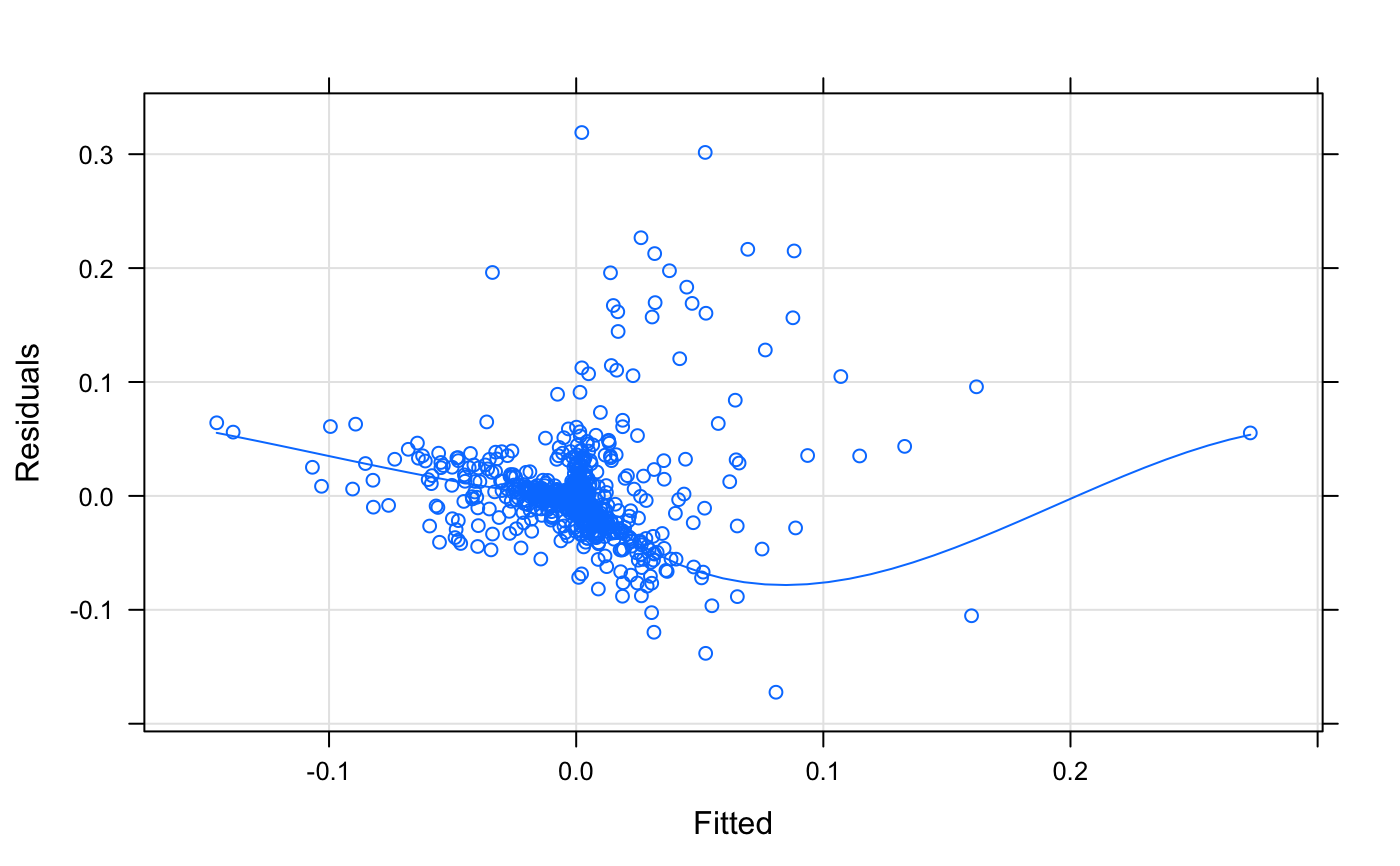
ordiresids.RdThe function provides plot.lm style diagnostic plots for
the results of constrained ordination from cca,
rda and capscale. Normally you do not need
these plots, because ordination is descriptive and does not
make assumptions on the distribution of the residuals. However, if
you permute residuals in significance tests (anova.cca),
you may be interested in inspecting that the residuals really are
exchangeable and independent of fitted values.
ordiresids(x, kind = c("residuals", "scale", "qqmath"),
   residuals = "working", type = c("p", "smooth", "g"),
   formula, ...)
Arguments
| x | |
|---|---|
| kind | The type of plot: |
| residuals | The kind of residuals and fitted values, with alternatives
|
| type | The type of plot. The argument is passed on to lattice functions. |
| formula | Formula to override the default plot. The formula can
contain items |
| ... | Other arguments passed to lattice functions. |
Details
The default plots are similar as in plot.lm, but they
use Lattice functions
xyplot and qqmath. The
alternatives have default formulae but these can be replaced by the
user. The elements available in formula or in the groups argument
are Fitted, Residuals, Species and Sites.
With residuals = "response" and residuals = "working"
the fitted values and residuals are found with functions
fitted.cca and residuals.cca. With
residuals = "standardized" the residuals are found with
rstandard.cca, and with residuals = "studentized"
they are found with rstudent.cca, and in both cases the
fitted values are standardized with sigma.cca.
Value
The function returns a Lattice object that can
displayed as plot.
See also
plot.lm, fitted.cca,
residuals.cca, rstandard.cca,
rstudent.cca, sigma.cca,
Lattice, xyplot,
qqmath.
Examples
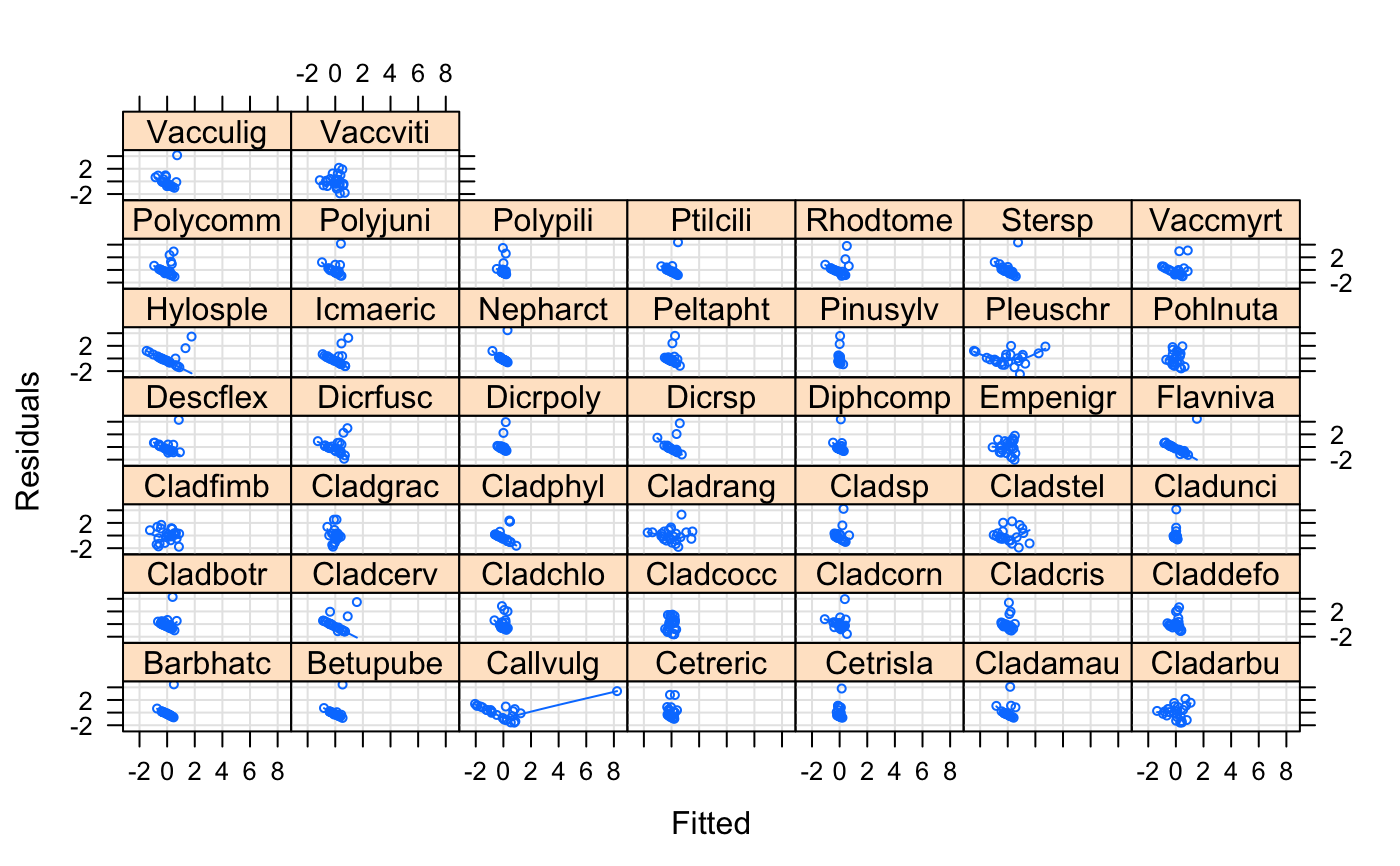
ordiresids(mod, formula = Residuals ~ Fitted | Species, residuals="standard", cex = 0.5)

