Standardization Methods for Community Ecology
decostand.RdThe function provides some popular (and effective) standardization methods for community ecologists.
decostand(x, method, MARGIN, range.global, logbase = 2, na.rm=FALSE, ...)
wisconsin(x)
Arguments
| x | Community data, a matrix-like object. |
|---|---|
| method | Standardization method. See Details for available options. |
| MARGIN | Margin, if default is not acceptable. |
| range.global | Matrix from which the range is found in
|
| logbase | The logarithm base used in |
| na.rm | Ignore missing values in row or column standardizations. |
| ... | Other arguments to the function (ignored). |
Details
The function offers following standardization methods for community data:
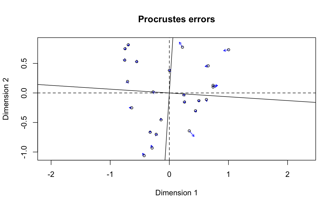
total: divide by margin total (defaultMARGIN = 1).max: divide by margin maximum (defaultMARGIN = 2).frequency: divide by margin total and multiply by the number of non-zero items, so that the average of non-zero entries is one (Oksanen 1983; defaultMARGIN = 2).normalize: make margin sum of squares equal to one (defaultMARGIN = 1).range: standardize values into range 0 ... 1 (defaultMARGIN = 2). If all values are constant, they will be transformed to 0.rank, rrank:rankreplaces abundance values by their increasing ranks leaving zeros unchanged, andrrankis similar but uses relative ranks with maximum 1 (defaultMARGIN = 1). Average ranks are used for tied values.standardize: scalexto zero mean and unit variance (defaultMARGIN = 2).pa: scalexto presence/absence scale (0/1).chi.square: divide by row sums and square root of column sums, and adjust for square root of matrix total (Legendre & Gallagher 2001). When used with the Euclidean distance, the distances should be similar to the Chi-square distance used in correspondence analysis. However, the results fromcmdscalewould still differ, since CA is a weighted ordination method (defaultMARGIN = 1).hellinger: square root ofmethod = "total"(Legendre & Gallagher 2001).log: logarithmic transformation as suggested by Anderson et al. (2006): \(\log_b (x) + 1\) for \(x > 0\), where \(b\) is the base of the logarithm; zeros are left as zeros. Higher bases give less weight to quantities and more to presences, andlogbase = Infgives the presence/absence scaling. Please note this is not \(\log(x+1)\). Anderson et al. (2006) suggested this for their (strongly) modified Gower distance (implemented asmethod = "altGower"invegdist), but the standardization can be used independently of distance indices.
Standardization, as contrasted to transformation, means that the entries are transformed relative to other entries.
All methods have a default margin. MARGIN=1 means rows (sites
in a normal data set) and MARGIN=2 means columns (species in a
normal data set).
Command wisconsin is a shortcut to common Wisconsin double
standardization where species (MARGIN=2) are first standardized
by maxima (max) and then sites (MARGIN=1) by
site totals (tot).
Most standardization methods will give nonsense results with
negative data entries that normally should not occur in the community
data. If there are empty sites or species (or constant with
method = "range"), many standardization will change these into
NaN.
Value
Returns the standardized data frame, and adds an attribute
"decostand" giving the name of applied standardization
"method".
Note
Common transformations can be made with standard R functions.
References
Anderson, M.J., Ellingsen, K.E. & McArdle, B.H. (2006) Multivariate dispersion as a measure of beta diversity. Ecology Letters 9, 683--693.
Legendre, P. & Gallagher, E.D. (2001) Ecologically meaningful transformations for ordination of species data. Oecologia 129, 271--280.
Oksanen, J. (1983) Ordination of boreal heath-like vegetation with principal component analysis, correspondence analysis and multidimensional scaling. Vegetatio 52, 181--189.
Examples
#> Callvulg Empenigr Rhodtome Vaccmyrt Vaccviti Pinusylv Descflex Betupube #> 1 1 1 1 1 1 1 1 #> Vacculig Diphcomp Dicrsp Dicrfusc Dicrpoly Hylosple Pleuschr Polypili #> 1 1 1 1 1 1 1 1 #> Polyjuni Polycomm Pohlnuta Ptilcili Barbhatc Cladarbu Cladrang Cladstel #> 1 1 1 1 1 1 1 1 #> Cladunci Cladcocc Cladcorn Cladgrac Cladfimb Cladcris Cladchlo Cladbotr #> 1 1 1 1 1 1 1 1 #> Cladamau Cladsp Cetreric Cetrisla Flavniva Nepharct Stersp Peltapht #> 1 1 1 1 1 1 1 1 #> Icmaeric Cladcerv Claddefo Cladphyl #> 1 1 1 1sptrans <- wisconsin(varespec) ## Chi-square: PCA similar but not identical to CA. ## Use wcmdscale for weighted analysis and identical results. sptrans <- decostand(varespec, "chi.square") plot(procrustes(rda(sptrans), cca(varespec)))
